Query Ingested Data
This page contains a walkthrough which guides you through the steps to query stored data on an active databases.
This walkthrough makes reference to data ingested through pipelines created in the other walkthroughs and deployed to the insights-demo database. Therefore, before you can create the queries in this walkthrough, ensure the insights-demo database is created, as described in the database documentation.
You must also build the pipelines to ingest the data. Details on these are provided on these pages:
Create a query
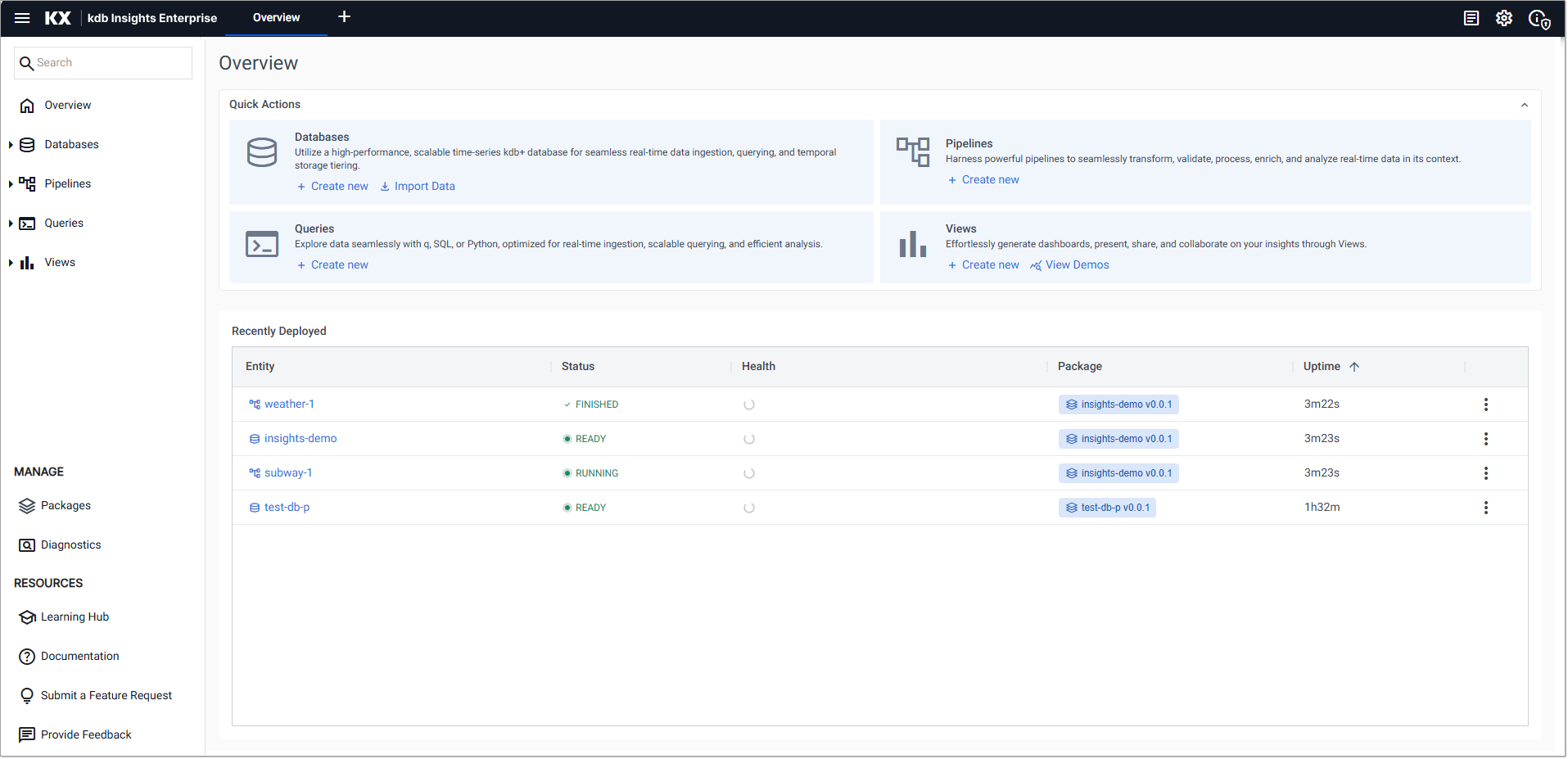
Click Create new under Queries on the Overview page.
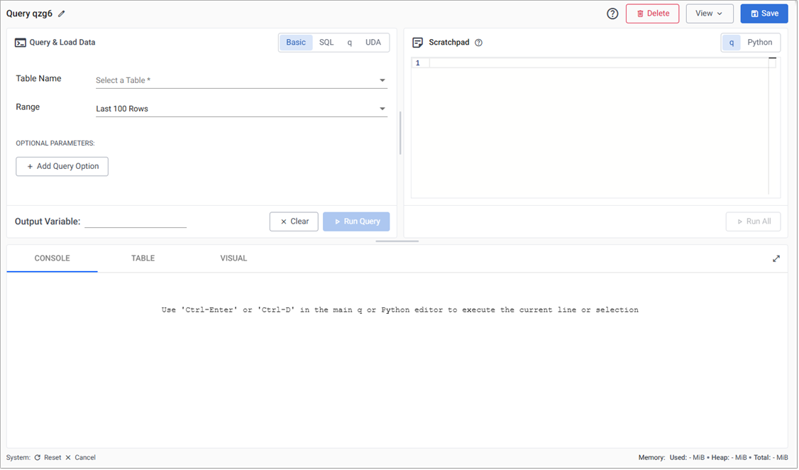
There is more than one method to query data from a database. Let's start with the Basic query in the Query Builder section of the screen, shown below. Click the SQL or q tab for details on how to run a query using SQL or q.
Basic
SQL
q
Basic is the simplest way to explore your data as it requires no coding experience
-
Select one of the available tables;
weather,crime,subway,health,taxifor the Table Name field. -
Define an Output variable.
-
Click Run Query to return data.
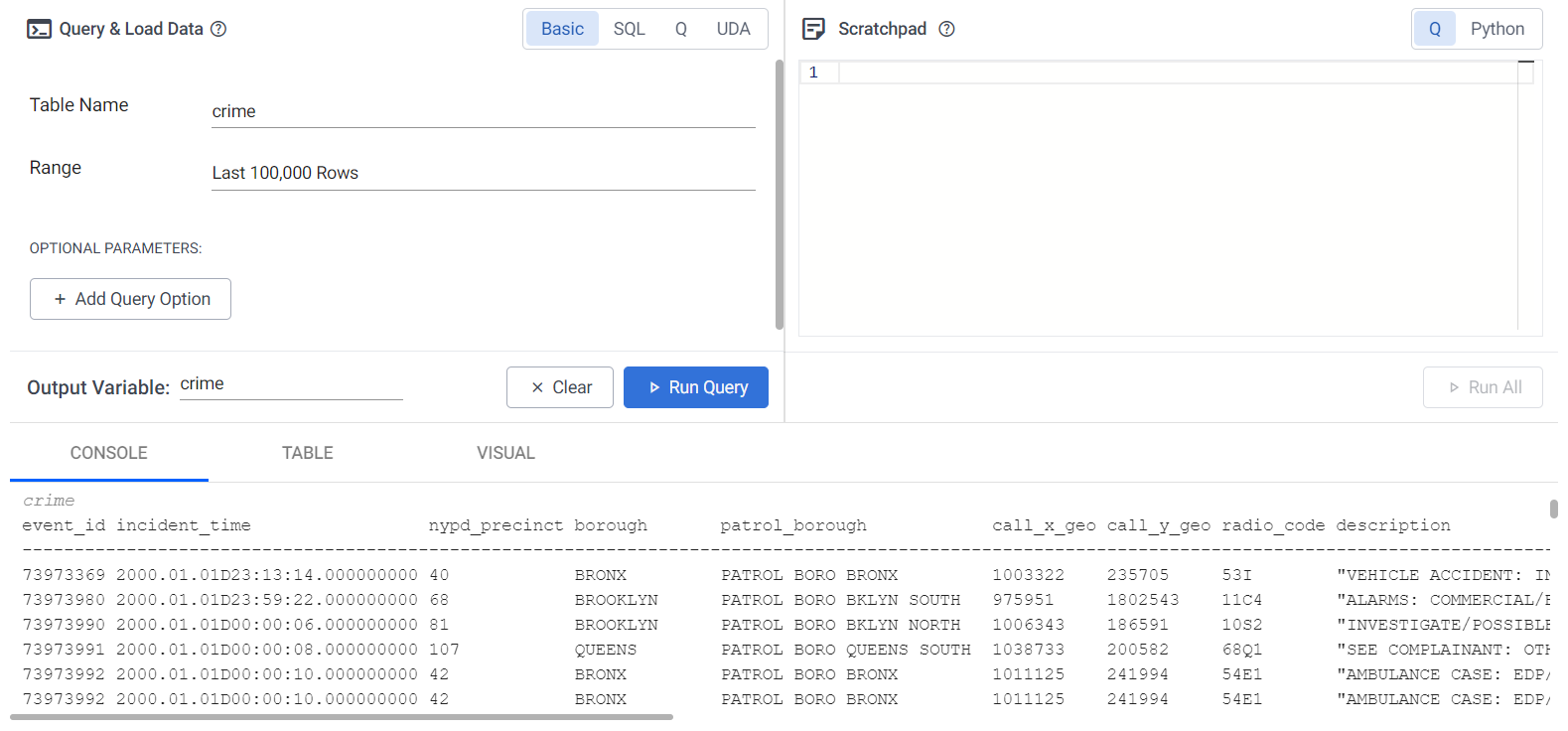
To query the insight-demo database with SQL:
-
Enter one of the sql queries from the following table, in the SQL tab.
Data
SQLqueryweatherselect * from weathercrimeselect * from crimesubwayselect * from subwayFor example, to see the number of events generated in the subway pipeline:
text
Copy`select * from subway` -
Define an Output Variable.
-
Click Run Query to generate results.
Note
This option only works when Query Environment(s) is enabled. Refer to System Information for details on how to check the status.
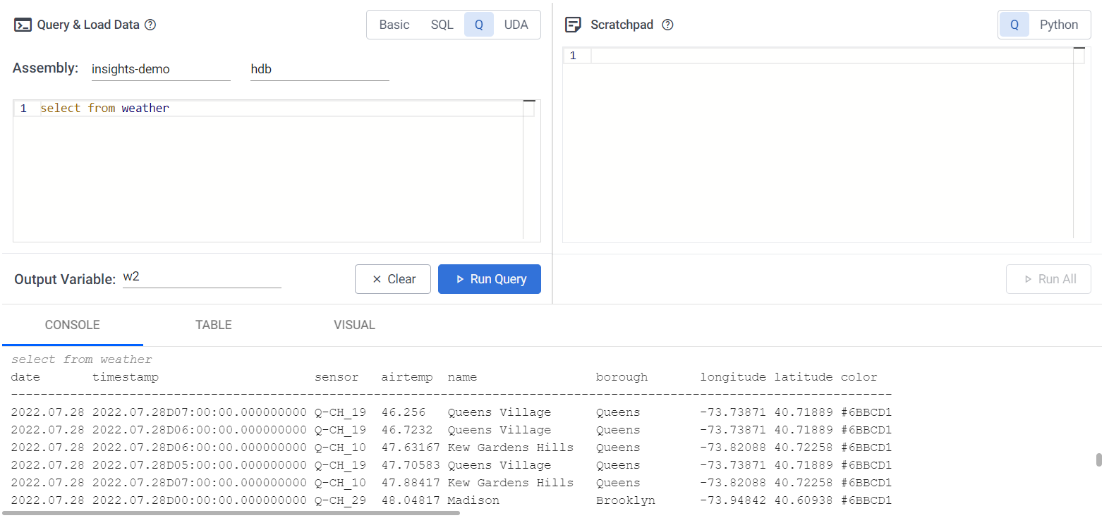
To query the insight-demo database with q:
-
Enter a query such as the following:
Data
qqueryweather
select from weather
crime
select from crime
subway
select from subway
-
Select insights-demo from the list of Assemblies and select an instance.
-
Define an Output Variable.
-
Click Run Query to generate results.
Note
You always need to define an Output Variable as this is used for querying in the scratchpad and is valid for the current session.
Ad-hoc queries using Scratchpad
You have the option to run additional data investigations in the Scratchpad with q or Python. Scratchpad queries must reference the Output Variable defined in the previous section. The following scratchpad queries reference the Output Variable defined in the previous section.
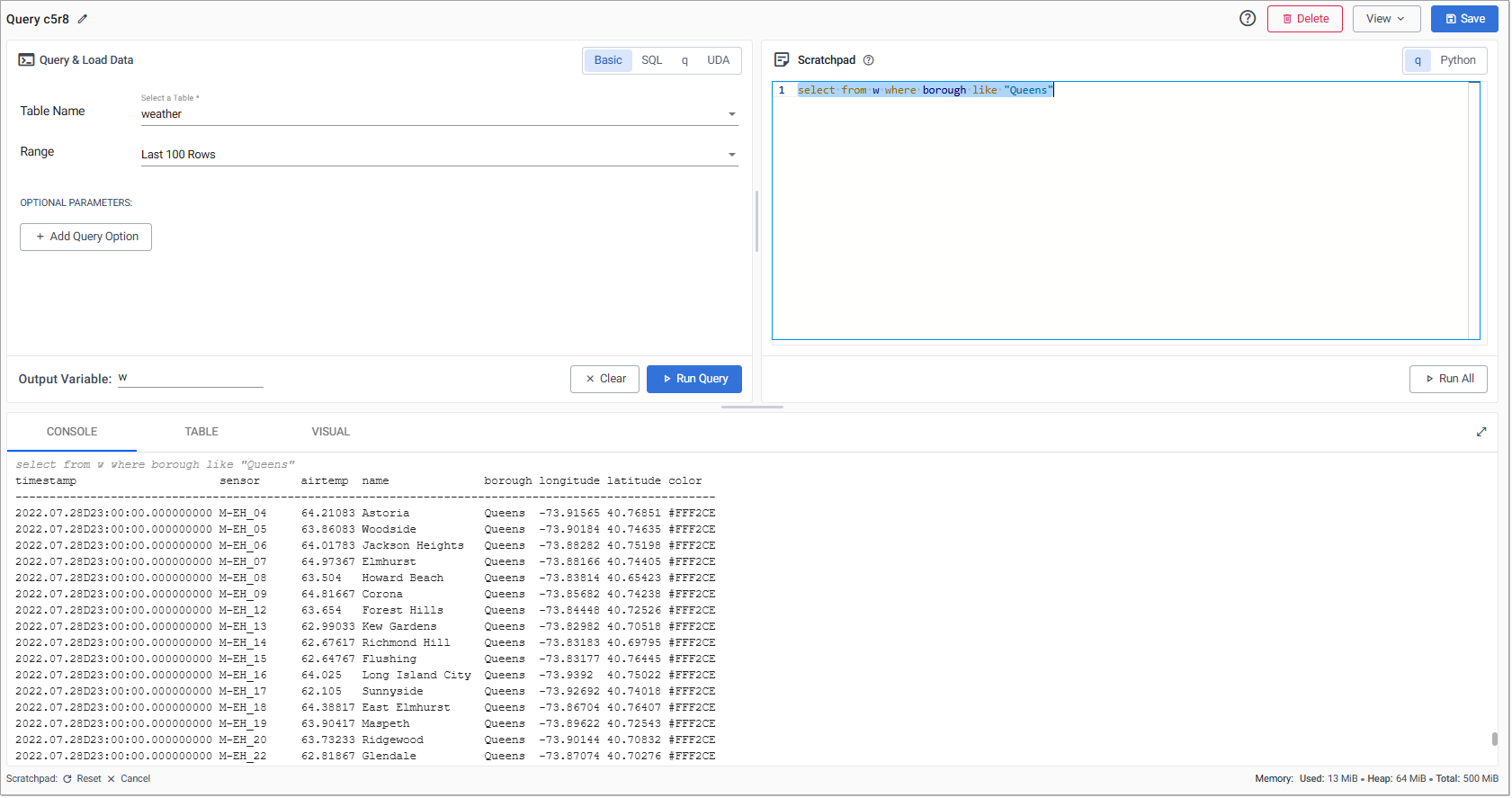
For example, to check the weather for the borough of Queens, where the basic query has been stored in the Output Variable w, enter the following query in the Scratchpad:
SQL
select from w where borough like "Queens"
-
Press Ctrl + D (Windows) or ⌘D (Mac) to evaluate the current line.
Warning
If you are using
python, only the first line of code is processed.Note
There is no requirement to use the Scratchpad to view data. The Scratchpad is for ad hoc analysis of the data and is done after
Run Queryis run.
View results
Once you have run queries either by clicking Run Query or Run Scratchpad the results are returned to lower portion of the screen in three tabs. Right-click inside the console window to clear results. For more information on each of these tabs see:
Note
The console shows results of the most recent query irrespective of the selected tab. When switching between tabs, re-run Run Query or Run Scratchpad to repopulate results for the selected tab.
Query subway data
The following sections provide instructions and code examples to help you query the Kafka subway data.
Event count
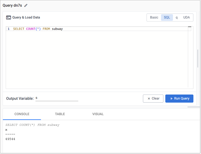
To count the number of subway journeys in the table, do the following.
-
Enter the following query in the
SQLtab:SQL
CopySELECT COUNT(*) FROM subway -
Define the Output Variable as
s. -
Click Run Query to execute the query. Rerun the query to get an updated value.
Filtering and visualizing
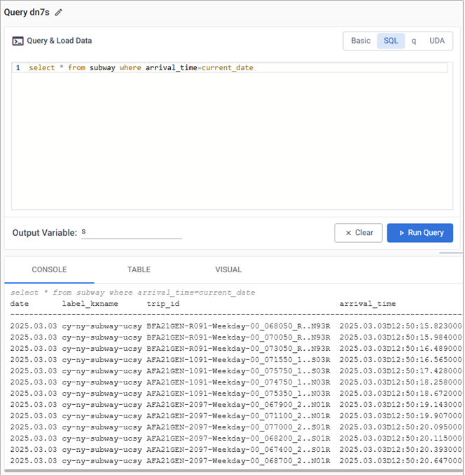
To get a subset of the data and perform further analysis using the Scratchpad:
-
Enter the following query in the
SQLtab.SQL
Copyselect * from subway where arrival_time=current_date -
Define the Output Variable as
s. -
Click Run Query.
Additional analysis, of today’s train data, can be performed against the s variable using the scratchpad. Querying in the scratchpad is more efficient than direct querying of the database and supports both q and python.
-
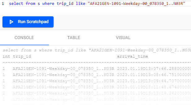
Enter the following query, in the Scratchpad and click Run All.
This pulls data for a selectedq
Copyselect from s where trip_id like "AFA21GEN-5108-Weekday-00_091350_5..N71R"trip_id. Change the value of thetrip_idto another if this example returns no results. -
Results are displayed in the tabs; Console, Table or Visual tabs.
-
In the Visual tab, set the y-axis to use
stop_sequenceand x-axis toarrival_timeto return a plot of journey times between each of the stops.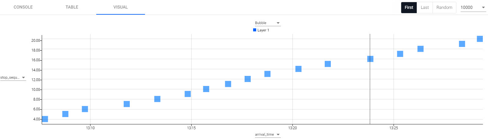
Note
Each time you change the results tab you must rerun the query.
Calculate average time between stops
You can calculate the average time between stops, as a baseline to determine percentage lateness.
-
In the scratchpad enter the following code, replacing the
trip-idwith the value you used in the previous section.The following screenshot shows this query in the scratchpad and the results in the Console.q
Copy`arrival_time`time_between_stops xcols
update time_between_stops:0^`second$arrival_time[i]-arrival_time[i-1] from
select from s
where trip_id like "AFA21GEN-1091-Weekday-00_138900_1..N03R"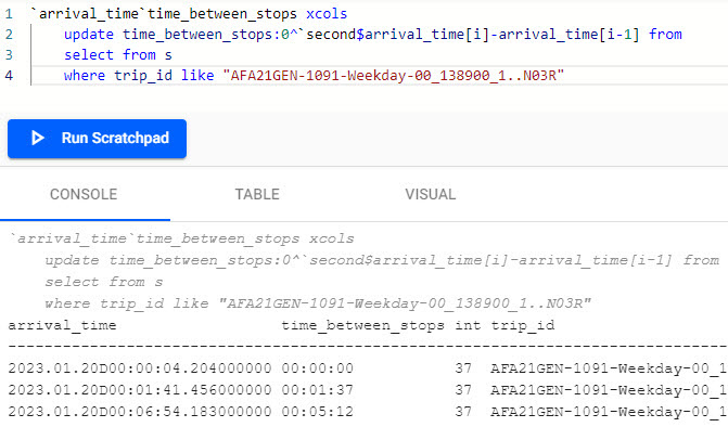
Note
 Understanding the q query
In the above query, the following
qelements are used:Element
Description
To reorder table columns
To replace nulls with zeros
To cast back to second datatype
To subtract each column from the previous one
If you run into an error on execution, check to ensure the correct code indentation is applied for
s3.Information
Use the Table tab to filter the results. For example, doing a column sort by clicking on the column header for the newly created variable
time_between_stopstoggles the longest and shortest stop for the selected trip.
Note
Each time you change the results tab you must rerun the query
Calculating percentage lateness for all trains
You can discover which trains were most frequently on time.
-
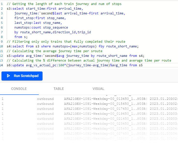
In the Scratchpad, replace any existing code with the following and click Run Scratchpad.
q
Copy// Getting the length of each train journey and num of stops
s3:select start_time:first arrival_time,
journey_time:`second$last arrival_time-first arrival_time,
first_stop:first stop_name,
last_stop:last stop_name,
numstops:count stop_sequence
by route_short_name,direction_id,trip_id
from s;
// Filtering only trains that fully completed their route
s4:select from s3 where numstops=(max;numstops) fby route_short_name;
// Calculating the average journey time per sroute
s5:update avg_time:`second$avg journey_time by route_short_name from s4;
// Calculating the % difference between actual journey time and average time per route
s6:update avg_vs_actual_pc:100*(journey_time-avg_time)%avg_time from s5Note
Understanding the q query?
In the above query, the following
qelements are used:Element
Description
To get first or last record
To subtract one column from another
To return the number of records
To group the results of table by column/s - similar to excel pivot
To filter results by a newly calculated field without needing to add it to table
To filter any records that equal the maximum value for that column
To cast back to second datatype
To perform multiplication
To perform division.
If you run into an error on execution, check to ensure the correct code indentation is applied.
Most punctual train
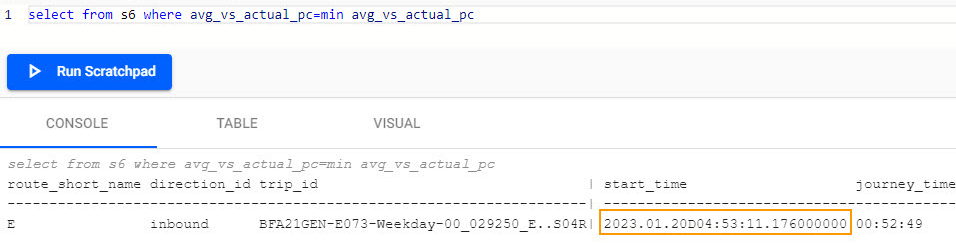
To calculate which train was most punctual:
-
In the Scratchpad, replace any existing code with the following and click Run Scratchpad
q
Copyselect from s6 where avg_vs_actual_pc=min avg_vs_actual_pcUsing min, the 04:53 route E train was the most punctual (your result will differ).
Visualize journey time
In the Visual tab, create a visualization for a single route.
-
In the Scratchpad, replace any existing code with the following and click Run Scratchpad.
q
Copy// Filtering for at only inbound trains on Route 1
select from s6 where route_short_name=`1 ,direction_id=`inbound -
Switch to a bar chart. Set the y-axis to
avg_vs_actual_pcand the x-axis tostart_timeto view results as shown below.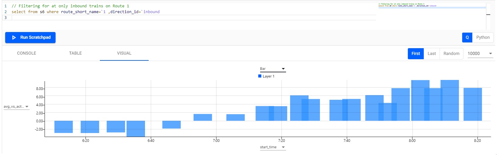
Distribution of journey times between stations
To assess the distribution of journey times between stations.
-
In the Scratchpad, replace any existing code with the following and click Run Scratchpad.
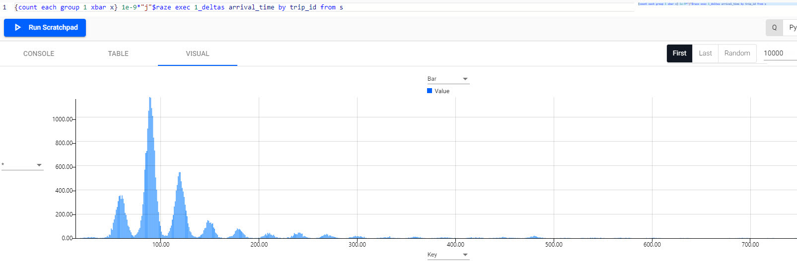
q
Copy{count each group 1 xbar x} 1e-9*"j"$raze exec 1_deltas arrival_time by trip_id from s -
From the histogram, you can see that the most common journey time between stations is 90 seconds.
Next steps
-
Read about how to visualize your data.
Further reading
Use the following links to learn more about specific topics mentioned in this page: