How to Use Dynamic Time Warping (DTW)
This guide shows how to use Dynamic Time Warping (DTW) with KDB.AI, via q, REST, and Python, to match patterns, measure similarity, and detect anomalies in time-series data.
Prerequisites
Before using DTW in KDB.AI:
-
Make sure your data is time-series vectors (for example, sensor readings, prices).
-
Include a timestamp or meaningful index to define sequence (recommended but not required).
-
Know how to use the KDB.AI Query API (Python, REST, or q).
-
Define patterns at query time, either manually or by sampling from prior data.
DTW is a flexible algorithm for comparing time-series sequences that may vary in timing or speed.
This guide walks through how to run DTW-based searches in KDB.AI, from defining your query pattern to comparing results across q, REST, and Python. It's suitable for use cases like shape-based pattern matching, temporal similarity, or anomaly detection in time-series data.
Overview of Steps
-
Prepare time-series vectors
-
Define a query pattern
-
Run a DTW similarity search
-
Visualize and compare matches
-
Compare DTW vs. TSS APIs
1. Prepare time-series vectors
Your dataset should include clean, regular time-series vectors for the feature(s) you wish to match - such as price, temperature, heart rate, or load. So that includes pre-processing (for example, handle missing values: interpolation, or deletion) and normalization, if necessary.
Python
# To extract time-series from data frame
data = df['price'].to_numpy(dtype='float64')
q
// To extract time-series from table
data:t[`price];
2. Define a query pattern
Create a query pattern representing the shape or behavior you're looking for. It can be a handcrafted sequence or sampled from historical data. In this example we used sampled historical data.
Python
# To extract length-128 queries from 3 different positions
extractedPositions = [2400, 6600, 9800]
size = 128
queryVectors = [data[posi:posi+size] for posi in extractedPositions]
q
extractedPositions:2400 6600 9800;
size:128;
extractedPositions +\: til size;
queryVectors:data extractedPositions +\: til size;
2b. (Optional) Warp/deform the query
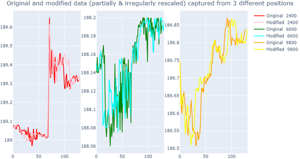
Warp the query to illustrate the power of DTW that deformed queries can still capture the original patterns. Now we apply rescaleFactors:(40#0.7),(60#1.4),(27#0.7) which means the first 40 spaces will be rescaled with ratio 0.7, and so on for the next 60spaces and next 27 spaces with rescale-ratio 1.4 and 0.7 (for example total 40+60+27+1 = 128 data).
Python
import numpy as np
import math

def deform_vector(v_ori, rescale_factors):
    v_ori = np.asarray(v_ori, dtype=float)

    rescale_factors = np.asarray(rescale_factors, dtype=float)

      if len(v_ori) != len(rescale_factors) + 1:
        raise ValueError("length of vOri should be 1 + length of rescaleFactors")

      def _reposition_two_values(v1, v2, p1, p2):
        ceil1, ceil2 = math.ceil(p1), math.ceil(p2)
        unit_inc     = (v2 - v1) / (p2 - p1)
        first_inc    = (ceil1 - p1) * unit_inc
        count        = ceil2 - ceil1               # how many integers we emit
        return v1 + first_inc + unit_inc * np.arange(count, dtype=float)

      v_last  = v_ori[-1]
      pos_new = np.concatenate(([0.0], np.cumsum(rescale_factors)))

      keep_idx = np.concatenate(([0],
np.where(np.diff(np.ceil(pos_new)) != 0)[0] + 1))
      pos_new_kept = pos_new[keep_idx]
      v_ori_kept   = v_ori[keep_idx]

      chunks = [_reposition_two_values(v_ori_kept[i], v_ori_kept[i + 1], pos_new_kept[i], pos_new_kept[i + 1]) for i in range(len(v_ori_kept) - 1)]
      return np.concatenate(chunks + [[v_last]]).astype(float)

rescale_factors = np.concatenate([ np.full(40, 0.7), np.full(60, 1.4), np.full(27, 0.7) ])

rng = np.random.default_rng(seed=42)

query_vectors = rng.random((3, len(rescale_factors) + 1)).cumsum(axis=1) # In case that you didn't define query_vectors above

qv0b = deform_vector(query_vectors[0], rescale_factors)

qv1b = deform_vector(query_vectors[1], rescale_factors)

qv2b = deform_vector(query_vectors[2], rescale_factors)

QueryVectorsModified = [qv0b, qv1b, qv2b]
q
deformVector:{[vOri;rescaleFactors]
 if[not count[vOri]~count[rescaleFactors]+1;'"length of vOri should be 1 + length of rescaleFactors"];
 repositioned2Values:{[valBefore1;valBefore2;posiBefore1;posiBefore2]
  ceil1:ceiling[posiBefore1];
  ceil2:ceiling[posiBefore2];
  unitIncrease:(valBefore2-valBefore1) % posiBefore2-posiBefore1;
  firstIncrease:(ceil1-posiBefore1)*unitIncrease;
  :valuesAfter:valBefore1+firstIncrease+unitIncrease*til ceil2 - ceil1;
  };

 vOriLast:last vOri;
 n:count[vOri]-1;
 posiNew:0f,sums rescaleFactors;

 posiKept:0,where (not 0= deltas (ceiling each posiNew));
 posiNew:posiNew[posiKept];
 vOri:vOri[posiKept];

 :"f"$((,/) repositioned2Values'[-1 _ vOri;1 _ vOri; -1 _ posiNew;1 _ posiNew]),vOriLast;
 };

rescaleFactors:(40#0.7),(60#1.4),(27#0.7);
queryVectors:(3 128)#(128*3)?1e; // In case that you didn't define queryVectors above

qv0b:deformVector[queryVectors[0];rescaleFactors];
qv1b:deformVector[queryVectors[1];rescaleFactors];
qv2b:deformVector[queryVectors[2];rescaleFactors];
QueryVectorsModified:(qv0b; qv1b; qv2b);
The deformed data will look like this:
3. Run a DTW similarity search
You can use DTW for similarity search just like TSS — the main difference is setting type: dtw.
Python
#DTW search with default parameters
result1 = table.search(vectors={'price': QueryVectorsModified}, n=50, type="dtw")[0]

#with RR (i.e. ratio of warping radius)
result2 = table.search(vectors={'price': QueryVectorsModified}, n=50, type="dtw", options={"RR":0.05})[0]
q
n:50;
tqry:enlist[`price]!enlist QueryVectorsModified;

// DTW search with default parameters
result1:gw(`search;`database`table`vectors`n`type!(`default;`myTable;tqry;n;`dtw));

// with RR (i.e. ratio of warping radius) and cutOff
result2:gw(`search;`database`table`vectors`n`type`options!(`default;`myTable;tqry;n;`dtw;(`RR`cutOff)!(0.05;0w)));
REST
curl -X POST http://localhost:8081/api/v2/databases/default/tables/mytable/search \
  --header 'Content-Type: application/json' \
  --data '{
    "vectors": {"price": [[0.1, 0.2, 0.3, 0.2, 0.1]]},
    "n": 50,
    "type": "dtw"
  }' | jq .

curl -X POST http://localhost:8081/api/v2/databases/default/tables/mytable/search \
  --header 'Content-Type: application/json' \
  --data '{
    "vectors": {"price": [[0.1, 0.2, 0.3, 0.2, 0.1]]},
    "n": 50,
    "type": "dtw",
    "options": {"RR" : 0.05}
  }' | jq .
4. Visualize and compare matches
You can visualize time-series matches and distance metrics using standard tools like matplotlib.
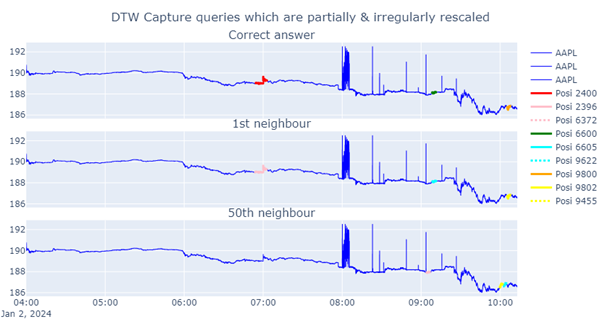
When patterns are deformed (for example, rescaled partially and irregularly), you can see that DTW's 1st neighbour succeeds in capturing all 3 patterns out of the 3 trials.
5. Compare DTW vs. TSS APIs
The only change required to switch from TSS to DTW is the type field:
Python
res_tss = table.search(vectors={'myScalar': queryVectorsModified}, n=50, type="tss", options={"returnMatches":True})[0]

res_dtw = table.search(vectors={'myScalar': queryVectorsModified}, n=50, type="dtw", options={"returnMatches":True})[0]
q
// TSS
r1:gw(`search;`database`table`vectors`n`type`options!(`default;`mytable;tqry;50;`tss;enlist[`returnMatches]!enlist 1b));

// DTW
r2:gw(`search;`database`table`vectors`n`type`options!(`default;`mytable;tqry;50;`dtw;enlist[`returnMatches]!enlist 1b));
REST
# TSS
curl -s -X POST http://localhost:8081/api/v2/databases/default/tables/trade/search \
--header 'Content-Type: application/json' \
--data '{
    "vectors":{"myScalar" : [[1.2,2.2,3.2]]},
    "n": 50,
    "type": "tss",
    "options":{"returnMatches" : true}
    }' | jq .

# DTW
curl -s -X POST http://localhost:8081/api/v2/databases/default/tables/trade/search \
--header 'Content-Type: application/json' \
--data '{
    "vectors":{"myScalar" : [[1.2,2.2,3.2]]},
    "n": 50,
    "type": "dtw",
    "options":{"returnMatches" : true }
    }' | jq .
Summary
In this guide, you:
-
Prepared normalized time-series vectors
-
Defined a pattern to search for
-
Performed DTW-based similarity search
-
Compared usage with TSS in q, REST, and Python
Performance tips
To improve DTW performance:
-
Use shorter query vectors where possible to reduce alignment overhead.
-
Set a
cutOffthreshold to skip matches above a certain distance. -
Apply a RR (ratio of warping radius, or of the Sakoe-Chiba band) to limit returned results to the most meaningful matches.
-
Pre-normalize your data to reduce noise and improve pattern clarity.
-
Benchmark DTW against TSS for your data shape and size - TSS is faster for aligned patterns.
-
Use vector indexing and partitions to reduce search scope in large datasets.
Next steps
-
Try DTW with sliding windows or event-aligned queries
-
Extend to multivariate DTW across multiple features
-
Use DTW for predictive modeling, anomaly detection, or clustering